A simple raytracing simulations using pyoptools
A typical raytracing simulation using the pyoptools.raytrace is
divided in the following steps:
Define an optical system
Define the rays to propagate
Introduce the rays in the system
Perform the propagation
Retrieve information about the propagation
Display results
For a simple example, let’s assume we want to simulate the propagation of a ray bundle through an spherical lens. For this case, an jupyter notebook will be used to perform the simulation:
$ jupyter notebook
After the jupyter notebook has started, it is needed to import the
pyoptools module. The following command will import all the
classes and functions defined in all submodules:
In [1]: from pyoptools.all import *
Now it is possible to begin the definition of the surfaces that will be used to create the lens:
In [2]: S1=Spherical(curvature=1/100., shape=Circular(radius=20.))

In [3]: S2=Spherical(curvature=1/200., shape=Circular(radius=20.))
The class pyoptools.raytrace.surface.Spherical receive in its constructor
2 arguments:
The first defines the curvature of the surface
The second defines the shape of the surface. In this case, both surfaces are limited by a circular aperture with a radius=20. Different shapes can be used. The predefined shapes can be found in
pyoptools.raytrace.shape.
Using this 2 surfaces it is possible to define and simulate our system, but there might be problems if the rays go into or out from the lens through the edges, so it is better to define an edge surface:
In [4]: S3=Cylinder(radius=20,length=6.997)
Now with all the required surfaces, we can assemble the lens:
In [5]: L1=Component(surflist=[(S1, (0, 0, -5), (0, 0, 0)), (S2, (0, 0, 5), (0, pi, 0)), (S3,(0,0,.509),(0,0,0))], material=schott["BK7"])
The class pyoptools.raytrace.component.Component receive in its
constructor 2 arguments:
The first argument surflist, gets a list of tuples:
surflist=[(S1, (0, 0, -5), (0, 0, 0)),
          (S2, (0, 0, 5), (0, pi, 0)),
          (S3,(0,0,.509),(0,0,0))]
Each tuple contains 3 objects. The first object is the surface to use, the second is a tuple (or list or numpy vector) containing the coordinates of the surface’s vertex in the component optical system, and the third is a tuple containing 3 rotation angles to be used to orientate the surface.
The second argument material receive information about the material
used to construct the lens. It can be a material defined in the
pyoptools.raytrace.mat_lib, a custom defined
pyoptools.raytrace.material.Material instance, or a floating point
number if the refraction index is constant for all wavelengths.
There are some predefined components, so there is no need to build all the
components from surfaces. Check the module pyoptools.raytrace.comp_lib
for a list of predefined components.
To be able top see some result, we will include one of this predefined components, that will act as a detector in our system:
In [6]: ccd=CCD(size=(10,10), transparent=False)
This line will define an opaque ccd-like detector, with a 10 by 10 size.
Now it is time to build the system. The system that will be created, has
a lens located in the coordinate (0,20,0), and the ccd detector located
in (0,150,0). Neither the ccd or the lens, will be rotated. By default,
all surfaces in pyoptools, are defined as having their optical axis aligned
to the Z axis, so the rotation tuple in this case is (0,0,0) for
both elements. This information is given in the complist argument:
In [7]: S=System(complist=[(L1, (0, 0, 20), (0, 0, 0)),(ccd, (0, 0, 150), (0, 0, 0))], n=1)
The n=1 argument, indicates that our system is surrounded by a media having a refraction index of 1 (vacuum).
Now we need to define a list containing the rays that will be propagated.
This can be done defining instances of the pyoptools.raytrace.ray.Ray
and appending them to a list, or using some predefined ray sources, that
are available in the module pyoptools.raytrace.ray.
For this example, a list containing 5 rays will be created:
In [8]: R=[Ray(pos=(0, 0, 0), dir=(0, 0, 1)), Ray(pos=(10, 0, 0), dir=(0, 0, 1)), Ray(pos=(-10, 0, 0), dir=(0, 0, 1)),Ray(pos=(0, 10, 0), dir=(0, 0, 1)), Ray(pos=(0, -10, 0), dir=(0, 0, 1)),]
now the rays are going to be added to the system, and propagated:
In [9]: S.ray_add(R)

In [10]: S.propagate()
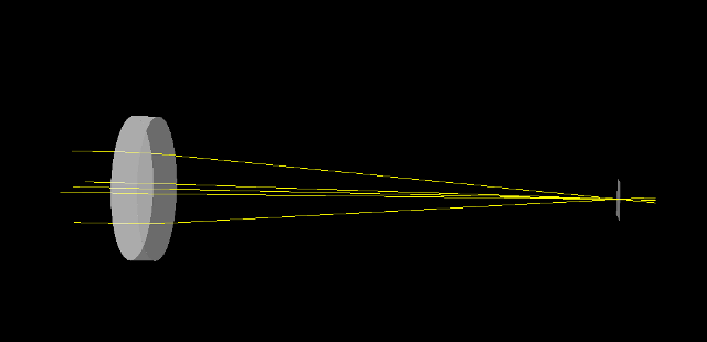
Finally, a 3D model of the system and the rays can be plotted:: diagram in the CCD will be plotted:
In[11]: Plot3D(S)
Note
To be able to visualize the results of the simulation in the Jupyter notebook, pythreejs plugin for jupyter must be installed as described in visualizing_pyoptools_in_jupyter
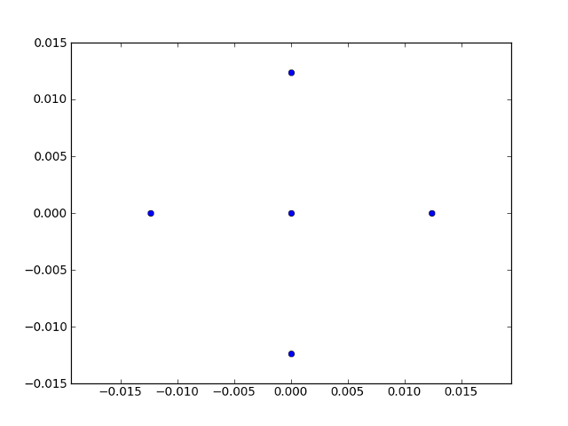
and and a spot can be obtained:
In[12]: spot_diagram(ccd)