Using predefined components with pyOpTools
Starting from surfaces to create components to define optical systems to run a simulation, can be very time consumming, for this reason pyOpTools has a growing library of predefined components. Some of these components, as well as some simple examples on how to use them to run simulation will be shown below.
[1]:
from pyoptools.all import *
from numpy import pi
Spherical lens
The most common optical systems are composed by spherical lenses, so pyOpTools have a SphericalLens helper class to create round-shaped sprerical lenses.
In this example a bi-convex lens with a diameter of 50mm (r=25mm) will be created. The curvature in both surfaces will be 1/100mm and the thickness at the center of the lens will be 10mm. The material used to simulate the lens is BK7 from the schoot catalog.
Using this lens a System is created. The position of the lens (the mid-point between the vertices) is the (0,0,100) coordinate. No rotation of the lens is made.
After the system is ready, a list of rays that will be propagated must be defined. In this example a list R, containing 5 rays is created. The origin of such Rays is defined as the coordinate (0,0,0). Each one has a different direction vector to create something similar to a point source located at the origin and aiming to the lens. The wavelength for all rays is defined as 650nm.
Note: In pyOpTools the wavelengths are defined in microns.
After the system and the ray beam are created, the later is added to the former, and the propagation calculation is performed.
The last Plot3d command creates an interactive 3D plot of the system and the propagated rays.
[2]:
L1 = SphericalLens(
radius=25,
curvature_s1=1.0 / 100.0,
curvature_s2=-1.0 / 100,
thickness=10,
material=material.schott["N-BK7"],
)
S = System(complist=[(L1, (0, 0, 100), (0, 0, 0))], n=1)
R = [
Ray(pos=(0, 0, 0), dir=(0, 0.2, 1), wavelength=0.650),
Ray(pos=(0, 0, 0), dir=(0, -0.2, 1), wavelength=0.650),
Ray(pos=(0, 0, 0), dir=(0.2, 0, 1), wavelength=0.650),
Ray(pos=(0, 0, 0), dir=(-0.2, 0, 1), wavelength=0.650),
Ray(pos=(0, 0, 0), dir=(0, 0, 1), wavelength=0.650),
]
S.ray_add(R)
S.propagate()
Plot3D(
S,
center=(0, 0, 100),
size=(300, 100),
scale=2,
rot=[(0, -pi / 2, 0), (pi / 20, -pi / 10, 0)],
)
/home/docs/checkouts/readthedocs.org/user_builds/pyoptools/envs/latest/lib/python3.12/site-packages/IPython/core/interactiveshell.py:3699: DeprecationWarning: The 'pos' keyword argument is deprecated and will be removed in a future version. Please use 'origin' instead.
exec(code_obj, self.user_global_ns, self.user_ns)
/home/docs/checkouts/readthedocs.org/user_builds/pyoptools/envs/latest/lib/python3.12/site-packages/IPython/core/interactiveshell.py:3699: DeprecationWarning: The 'dir' keyword argument is deprecated and will be removed in a future version. Please use 'direction' instead.
exec(code_obj, self.user_global_ns, self.user_ns)
[2]:
Besides the SphericalLens, pyOptools has classes to create the following lenses:
CCD
Most of the time it is needed a way to get information, such a spot diagram at a certain place in the system after running a simulation. pyOpTools define the CCD component for this task. Its main use is to capture ray information ar a given place in the optical system. Several CCD instances can be used in the same setup.
In the next example a system made up from a CCD with a size of 10mm X 10 mm and an spherical lens will be created and simulated:
[3]:
L1 = SphericalLens(
radius=25,
curvature_s1=1.0 / 100.0,
curvature_s2=-1.0 / 100,
thickness=10,
material=material.schott["N-BK7"],
)
SEN1 = CCD(size=(10, 10))
S = System(complist=[(L1, (0, 0, 200), (0, 0, 0)), (SEN1, (0, 0, 400), (0, 0, 0))], n=1)
R = [
Ray(pos=(0, 0, 0), dir=(0, 0.1, 1), wavelength=0.650),
Ray(pos=(0, 0, 0), dir=(0, -0.1, 1), wavelength=0.650),
Ray(pos=(0, 0, 0), dir=(0.1, 0, 1), wavelength=0.650),
Ray(pos=(0, 0, 0), dir=(-0.1, 0, 1), wavelength=0.650),
Ray(pos=(0, 0, 0), dir=(0, 0, 1), wavelength=0.650),
]
S.ray_add(R)
S.propagate()
Plot3D(
S,
center=(0, 0, 200),
size=(450, 100),
scale=2,
rot=[(0, -pi / 2, 0), (pi / 20, -pi / 10, 0)],
)
/home/docs/checkouts/readthedocs.org/user_builds/pyoptools/envs/latest/lib/python3.12/site-packages/IPython/core/interactiveshell.py:3699: DeprecationWarning: The 'pos' keyword argument is deprecated and will be removed in a future version. Please use 'origin' instead.
exec(code_obj, self.user_global_ns, self.user_ns)
/home/docs/checkouts/readthedocs.org/user_builds/pyoptools/envs/latest/lib/python3.12/site-packages/IPython/core/interactiveshell.py:3699: DeprecationWarning: The 'dir' keyword argument is deprecated and will be removed in a future version. Please use 'direction' instead.
exec(code_obj, self.user_global_ns, self.user_ns)
/home/docs/checkouts/readthedocs.org/user_builds/pyoptools/envs/latest/lib/python3.12/site-packages/IPython/core/interactiveshell.py:3699: DeprecationWarning: The 'pos' keyword argument is deprecated and will be removed in a future version. Please use 'origin' instead.
exec(code_obj, self.user_global_ns, self.user_ns)
/home/docs/checkouts/readthedocs.org/user_builds/pyoptools/envs/latest/lib/python3.12/site-packages/IPython/core/interactiveshell.py:3699: DeprecationWarning: The 'dir' keyword argument is deprecated and will be removed in a future version. Please use 'direction' instead.
exec(code_obj, self.user_global_ns, self.user_ns)
/home/docs/checkouts/readthedocs.org/user_builds/pyoptools/envs/latest/lib/python3.12/site-packages/IPython/core/interactiveshell.py:3699: DeprecationWarning: The 'pos' keyword argument is deprecated and will be removed in a future version. Please use 'origin' instead.
exec(code_obj, self.user_global_ns, self.user_ns)
/home/docs/checkouts/readthedocs.org/user_builds/pyoptools/envs/latest/lib/python3.12/site-packages/IPython/core/interactiveshell.py:3699: DeprecationWarning: The 'dir' keyword argument is deprecated and will be removed in a future version. Please use 'direction' instead.
exec(code_obj, self.user_global_ns, self.user_ns)
/home/docs/checkouts/readthedocs.org/user_builds/pyoptools/envs/latest/lib/python3.12/site-packages/IPython/core/interactiveshell.py:3699: DeprecationWarning: The 'pos' keyword argument is deprecated and will be removed in a future version. Please use 'origin' instead.
exec(code_obj, self.user_global_ns, self.user_ns)
/home/docs/checkouts/readthedocs.org/user_builds/pyoptools/envs/latest/lib/python3.12/site-packages/IPython/core/interactiveshell.py:3699: DeprecationWarning: The 'dir' keyword argument is deprecated and will be removed in a future version. Please use 'direction' instead.
exec(code_obj, self.user_global_ns, self.user_ns)
/home/docs/checkouts/readthedocs.org/user_builds/pyoptools/envs/latest/lib/python3.12/site-packages/IPython/core/interactiveshell.py:3699: DeprecationWarning: The 'pos' keyword argument is deprecated and will be removed in a future version. Please use 'origin' instead.
exec(code_obj, self.user_global_ns, self.user_ns)
/home/docs/checkouts/readthedocs.org/user_builds/pyoptools/envs/latest/lib/python3.12/site-packages/IPython/core/interactiveshell.py:3699: DeprecationWarning: The 'dir' keyword argument is deprecated and will be removed in a future version. Please use 'direction' instead.
exec(code_obj, self.user_global_ns, self.user_ns)
[3]:
After the rays propagation is finished, it is possible to plot the spot diagram of the CCD. In this case it can be seen that the CCD is not located close to the image plane.
[4]:
spot_diagram(SEN1)
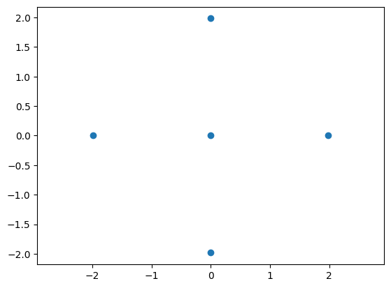
The sensor has an attribute called hit_list. This is a list containing a set of tuples with the coordinates of each hit point, and the ray that hitted at this point. In the following example, the coordinates of the hit point is printed:
[5]:
for C, R in SEN1.hit_list:
print(C)
(0.0, -1.9834327142873072, 0.0)
(0.0, 1.9834327142873072, 0.0)
(-1.9834327142873072, 0.0, 0.0)
(1.9834327142873072, 0.0, 0.0)
(0.0, 0.0, 0.0)
Stop
When creating optical systems, some time it is needed to put stops or apertures in the optical path. The Stop object was created for this purpose.
In the following example an aperture whose external shape is a circle of 20 mm radius with an aperture shape (the hole) also circular but with 5mm radius will be placed in front of the lens.
Warning: In the 3D plot the stop aperture is not shown. This is something to be fixed. Still the simulation works fine.
[6]:
L1 = SphericalLens(
radius=25,
curvature_s1=1.0 / 100.0,
curvature_s2=-1.0 / 100,
thickness=10,
material=material.schott["N-BK7"],
)
SEN1 = CCD(size=(10, 10))
ST1 = Stop(shape=Circular(radius=20), ap_shape=Circular(radius=5))
S = System(
complist=[
(L1, (0, 0, 200), (0, 0, 0)),
(SEN1, (0, 0, 400), (0, 0, 0)),
(ST1, (0, 0, 180), (0, 0, 0)),
],
n=1,
)
R = [
Ray(pos=(0, 0, 0), dir=(0, 0.1, 1), wavelength=0.650),
Ray(pos=(0, 0, 0), dir=(0, -0.1, 1), wavelength=0.650),
Ray(pos=(0, 0, 0), dir=(0.1, 0, 1), wavelength=0.650),
Ray(pos=(0, 0, 0), dir=(-0.1, 0, 1), wavelength=0.650),
Ray(pos=(0, 0, 0), dir=(0, 0, 1), wavelength=0.650),
]
S.ray_add(R)
S.propagate()
Plot3D(
S,
center=(0, 0, 200),
size=(450, 100),
scale=2,
rot=[(0, -pi / 2, 0), (pi / 20, -pi / 10, 0)],
)
/home/docs/checkouts/readthedocs.org/user_builds/pyoptools/envs/latest/lib/python3.12/site-packages/IPython/core/interactiveshell.py:3699: DeprecationWarning: The 'pos' keyword argument is deprecated and will be removed in a future version. Please use 'origin' instead.
exec(code_obj, self.user_global_ns, self.user_ns)
/home/docs/checkouts/readthedocs.org/user_builds/pyoptools/envs/latest/lib/python3.12/site-packages/IPython/core/interactiveshell.py:3699: DeprecationWarning: The 'dir' keyword argument is deprecated and will be removed in a future version. Please use 'direction' instead.
exec(code_obj, self.user_global_ns, self.user_ns)
/home/docs/checkouts/readthedocs.org/user_builds/pyoptools/envs/latest/lib/python3.12/site-packages/IPython/core/interactiveshell.py:3699: DeprecationWarning: The 'pos' keyword argument is deprecated and will be removed in a future version. Please use 'origin' instead.
exec(code_obj, self.user_global_ns, self.user_ns)
/home/docs/checkouts/readthedocs.org/user_builds/pyoptools/envs/latest/lib/python3.12/site-packages/IPython/core/interactiveshell.py:3699: DeprecationWarning: The 'dir' keyword argument is deprecated and will be removed in a future version. Please use 'direction' instead.
exec(code_obj, self.user_global_ns, self.user_ns)
/home/docs/checkouts/readthedocs.org/user_builds/pyoptools/envs/latest/lib/python3.12/site-packages/IPython/core/interactiveshell.py:3699: DeprecationWarning: The 'pos' keyword argument is deprecated and will be removed in a future version. Please use 'origin' instead.
exec(code_obj, self.user_global_ns, self.user_ns)
/home/docs/checkouts/readthedocs.org/user_builds/pyoptools/envs/latest/lib/python3.12/site-packages/IPython/core/interactiveshell.py:3699: DeprecationWarning: The 'dir' keyword argument is deprecated and will be removed in a future version. Please use 'direction' instead.
exec(code_obj, self.user_global_ns, self.user_ns)
/home/docs/checkouts/readthedocs.org/user_builds/pyoptools/envs/latest/lib/python3.12/site-packages/IPython/core/interactiveshell.py:3699: DeprecationWarning: The 'pos' keyword argument is deprecated and will be removed in a future version. Please use 'origin' instead.
exec(code_obj, self.user_global_ns, self.user_ns)
/home/docs/checkouts/readthedocs.org/user_builds/pyoptools/envs/latest/lib/python3.12/site-packages/IPython/core/interactiveshell.py:3699: DeprecationWarning: The 'dir' keyword argument is deprecated and will be removed in a future version. Please use 'direction' instead.
exec(code_obj, self.user_global_ns, self.user_ns)
/home/docs/checkouts/readthedocs.org/user_builds/pyoptools/envs/latest/lib/python3.12/site-packages/IPython/core/interactiveshell.py:3699: DeprecationWarning: The 'pos' keyword argument is deprecated and will be removed in a future version. Please use 'origin' instead.
exec(code_obj, self.user_global_ns, self.user_ns)
/home/docs/checkouts/readthedocs.org/user_builds/pyoptools/envs/latest/lib/python3.12/site-packages/IPython/core/interactiveshell.py:3699: DeprecationWarning: The 'dir' keyword argument is deprecated and will be removed in a future version. Please use 'direction' instead.
exec(code_obj, self.user_global_ns, self.user_ns)
[6]:
Block
pyOpTools has also an optical glass block as predefined component.
In the next example it will be show hot a ray is displaced laterally by the refraction in a glass block.
[7]:
BL1 = Block(size=(15, 15, 30), material=material.schott["N-BK7"])
S = System(
complist=[
(BL1, (0, 0, 50), (pi / 8, 0, 0)),
]
)
S.ray_add(Ray(pos=(0, 0, 0), dir=(0, 0, 1), wavelength=0.650))
S.propagate()
Plot3D(S, center=(0, 0, 50), size=(100, 50), scale=5, rot=[(0, -pi / 2, 0)])
/home/docs/checkouts/readthedocs.org/user_builds/pyoptools/envs/latest/lib/python3.12/site-packages/IPython/core/interactiveshell.py:3699: DeprecationWarning: The 'pos' keyword argument is deprecated and will be removed in a future version. Please use 'origin' instead.
exec(code_obj, self.user_global_ns, self.user_ns)
/home/docs/checkouts/readthedocs.org/user_builds/pyoptools/envs/latest/lib/python3.12/site-packages/IPython/core/interactiveshell.py:3699: DeprecationWarning: The 'dir' keyword argument is deprecated and will be removed in a future version. Please use 'direction' instead.
exec(code_obj, self.user_global_ns, self.user_ns)
[7]:
Right Angle Prism
Right angle prisms are also among the pyOpTools predefined components. In the next example a RightAnglePrism will be used as a retroreflector.
[8]:
RAP1 = RightAnglePrism(width=20, height=20, material=material.schott["N-BK7"])
S = System(
complist=[
(RAP1, (0, 0, 50), (0, -3 * pi / 4, 0)),
]
)
S.ray_add(Ray(pos=(10, 0, 0), dir=(0, 0, 1), wavelength=0.650))
S.propagate()
Plot3D(S, center=(0, 0, 50), size=(100, 50), scale=5, rot=[(pi / 2, 0, 0)])
/home/docs/checkouts/readthedocs.org/user_builds/pyoptools/envs/latest/lib/python3.12/site-packages/IPython/core/interactiveshell.py:3699: DeprecationWarning: The 'pos' keyword argument is deprecated and will be removed in a future version. Please use 'origin' instead.
exec(code_obj, self.user_global_ns, self.user_ns)
/home/docs/checkouts/readthedocs.org/user_builds/pyoptools/envs/latest/lib/python3.12/site-packages/IPython/core/interactiveshell.py:3699: DeprecationWarning: The 'dir' keyword argument is deprecated and will be removed in a future version. Please use 'direction' instead.
exec(code_obj, self.user_global_ns, self.user_ns)
[8]:
Besides the RightAnglePrism, pyOptools has classes to create the following prisms:
Mirrors
pyOpTools have 2 different predefined mirror types, the RectMirror and the RoundMirror. Both this mirrors can be 100% reflective or partially reflective (beam splitters).
The next example show a mirror and a beam splitter in the same setup.
[9]:
M1 = RectMirror(
size=(25.0, 25.0, 3.0), reflectivity=0.5, material=material.schott["N-BK7"]
)
M2 = RoundMirror(
radius=12.5, thickness=3, reflectivity=1.0, material=material.schott["N-BK7"]
)
S = System(
complist=[
(M1, (0, 0, 50), (pi / 4, 0, 0)),
(M2, (0, 50, 50), (pi / 4, 0, 0)),
],
n=1,
)
S.ray_add(Ray(pos=(0, 0, 0), dir=(0, 0, 1), wavelength=0.650))
S.propagate()
Plot3D(S, center=(0, 25, 50), size=(150, 100), scale=4, rot=[(0, -pi / 2, 0)])
/home/docs/checkouts/readthedocs.org/user_builds/pyoptools/envs/latest/lib/python3.12/site-packages/IPython/core/interactiveshell.py:3699: DeprecationWarning: The 'pos' keyword argument is deprecated and will be removed in a future version. Please use 'origin' instead.
exec(code_obj, self.user_global_ns, self.user_ns)
/home/docs/checkouts/readthedocs.org/user_builds/pyoptools/envs/latest/lib/python3.12/site-packages/IPython/core/interactiveshell.py:3699: DeprecationWarning: The 'dir' keyword argument is deprecated and will be removed in a future version. Please use 'direction' instead.
exec(code_obj, self.user_global_ns, self.user_ns)
[9]:
BeamSplittingCube
Besides mirrors that behave as beam splitters, pyOpTool has a class to simulate BeamSplittingCube. The next code show an example of its use.
[10]:
BS = BeamSplittingCube()
S = System(
complist=[
(BS, (0, 0, 50), (0, 0, 0)),
]
)
S.ray_add(Ray(pos=(0, 0, 0), dir=(0, 0, 1), wavelength=0.650))
S.propagate()
Plot3D(S, center=(0, 0, 50), size=(100, 150), scale=5, rot=[(pi / 2, 0, 0)])
/home/docs/checkouts/readthedocs.org/user_builds/pyoptools/envs/latest/lib/python3.12/site-packages/IPython/core/interactiveshell.py:3699: DeprecationWarning: The 'pos' keyword argument is deprecated and will be removed in a future version. Please use 'origin' instead.
exec(code_obj, self.user_global_ns, self.user_ns)
/home/docs/checkouts/readthedocs.org/user_builds/pyoptools/envs/latest/lib/python3.12/site-packages/IPython/core/interactiveshell.py:3699: DeprecationWarning: The 'dir' keyword argument is deprecated and will be removed in a future version. Please use 'direction' instead.
exec(code_obj, self.user_global_ns, self.user_ns)
[10]:
Warning: In older versions of pyOpTools BeamSplittingCube was misspelled. Please use the correct spelling.