Warning

There is an issue with the generation of documentation from notebooks, such as this page, that causes interactive plots generated using the Plot3D function to appear incorrect. The examples should produce correct 3D plots when executed directly in Jupyter Lab.

A more complex example

In this example we will simulate a simple autocolimator system.

The autocolimator system will be made of a point source (R), a beam splitting cube (BS), a colimator lens (L), and a CCD (C).

In this first example, this will be used to check if a mirror (M1) is parallel to the optical axis.

from pyoptools.all import *
from numpy import pi

R=point_source_c(span=(0.06,0.06),num_rays=(5,5),wavelength=.65)
BS=BeamSplittingCube(size=25,reflectivity=.5,material=material.schott["N-BK7"])
L=library.Edmund.get("32494")
C=CCD()
M1= RectMirror(size=(25, 25, 5),material=material.schott["N-BK7"], reflectivity=1.)

S=System(complist=[(C,(20,0,20),(0,pi/2,0)),(BS,(0,0,20),(0,0,0)),(L,(0,0,158.5),(0,-pi,0)),(M1,(0,0,170),(0,0,0))],n=1.)


S.ray_add(R)
S.propagate()

/home/docs/checkouts/readthedocs.org/user_builds/pyoptools/envs/latest/lib/python3.7/site-packages/pyoptools-0.2.0-py3.7-linux-x86_64.egg/pyoptools/raytrace/library/library.py:159: DeprecationWarning: This method is deprecated, you can use dictionary-style accessinstead
  DeprecationWarning,

Plot3D(S,center=(0,0,300), size=(600,100),scale=2,rot=[(0,0,-3*pi/8),(0,3*pi/8,0)])

/home/docs/checkouts/readthedocs.org/user_builds/pyoptools/envs/latest/lib/python3.7/site-packages/ipywidgets/widgets/widget.py:501: DeprecationWarning: Passing unrecognized arguments to super(MeshPhongMaterial).__init__(ambient='#050505').
object.__init__() takes exactly one argument (the instance to initialize)
This is deprecated in traitlets 4.2.This error will be raised in a future release of traitlets.
  super().__init__(**kwargs)

In this example, the ray trace proceesd as follow:

1. 25 rays come out from a the point source (R)
2. They enter the beam splitting cube (BS), and propagate to the BS reflective surface. In the first interface of BS the rays get diffracted.
3. In the reflective surface, the original rays continue propagating, and a new set of rays (reflected) get created.
4. The set of reflected rays get propagated out of the cube, and do not get propagated anymore as there are no optical components they can intersect.
5. The transmitted rays get propagated out of the cube, until they intersect the lens (L).
6. The rays get propagated through the lens. At each lens surface, the rays get refracted taking in to account the incidence angle, and the refraction index at each side of the surface. Note: This happens at all surface intersection, at all components.
7. The rays get propagated until they hit the reflective surface at the mirror, and bounce back, propagating again in the lens direction.
8. The rays get propagated through the lens and into the BS.
9. In the reflective surface of the BS a new set of reflected rays get created, and are propagated in the CCD direction.
10. the transmitted rays get propagated out of the BS and overlap the point source.

From the interactive raytrace plot, one can get an idea about what is going on, but most of the time we need to see how the ray intersect a surface. In this case, we can get an spot diagram from the CCD as shown in the next plot.

%pylab inline
spot_diagram(C)

Populating the interactive namespace from numpy and matplotlib

/home/docs/checkouts/readthedocs.org/user_builds/pyoptools/envs/latest/lib/python3.7/site-packages/IPython/core/magics/pylab.py:160: UserWarning: pylab import has clobbered these variables: ['sqrt', 'Polygon', 'cross', 'unwrap']
`%matplotlib` prevents importing * from pylab and numpy
  "\n`%matplotlib` prevents importing * from pylab and numpy"

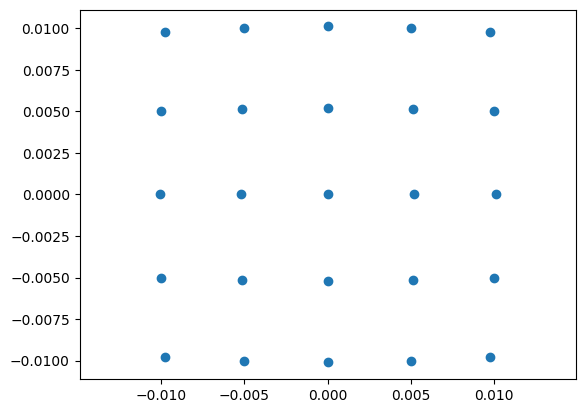
If the lens was ideal, and the distance between the lens and the point source was adequatelly adjusted, the spot diagram would show all the 25 rays hitting at exact the same coordinates in the CCD. But as we are simulating a “real” doublet, we have a cube that introduces some spherical aberration in the path, and the distance was optimized in .5 mm steps, we get a spot in the CCD that is about 20 um in diameter, but as expected the center of such spot is the (0mm, 0mm) coordinate f the CCD.

In the next example the mirror will be tilted 10 urads

R=point_source_c(span=(0.06,0.06),num_rays=(5,5),wavelength=.65)
BS=BeamSplittingCube(size=25,reflectivity=.5,material=material.schott["N-BK7"])
L=library.Edmund.get("32494")
C=CCD()
M1= RectMirror(size=(25, 25, 5),material=material.schott["N-BK7"], reflectivity=1.)

S=System(complist=[(C,(20,0,20),(0,pi/2,0)),(BS,(0,0,20),(0,0,0)),(L,(0,0,158.5),(0,-pi,0)),(M1,(0,0,170),(10.E-6,0,0))],n=1.)


S.ray_add(R)
S.propagate()

spot_diagram(C)

/home/docs/checkouts/readthedocs.org/user_builds/pyoptools/envs/latest/lib/python3.7/site-packages/pyoptools-0.2.0-py3.7-linux-x86_64.egg/pyoptools/raytrace/library/library.py:159: DeprecationWarning: This method is deprecated, you can use dictionary-style accessinstead
  DeprecationWarning,

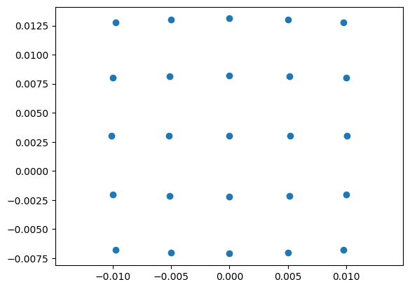
In this case we see that the spot is hitting the CCD approximately at (0mm, 0.0025 mm).

Some times getting an approximate position of the center of the spot from a plot is not enough. In such cases we can use the hit_list property from the CCD. From this list we can get the intersection point of each ray and for example use the average in X and in Y to estimate the spot centroid position.

cx=0.
cy=0.

for c,r in C.hit_list:
    cx=cx+c[0]
    cy=cy+c[1]

cx=cx/25
cy=cy/25

print("CMX",cx,"CMY",cy)

CMX 6.07784655937138e-15 CMY 0.002998219837423827

In this case, the resulting spot diagram is similar to the previous one, but we can see the central spot is not located at the origin of the CCD anymore, but at the coordinate (0 mm, 0.003 mm)

In the ideal case, taking in to account the reported focal length of the lens, and the tilting of the mirror, the coorditates of the point should be

f=150.
alpha=10e-6
cy_=f*2.*alpha
print("CMY-Estimated",cy_)

CMY-Estimated 0.003

As we can see, the estimated value correspond very well with the simulation.